Learning procedure

We work with numerically generated training trajectories that we denote by

(1)\[\begin{align} \{(x_i,y_i^2,...,y_i^M)\}_{i=1,...,N}. \end{align}\]

To obtain an approximation of the Hamiltonian \(H\), we define a parametric model \(H_{\Theta}\) and look for a \(\Theta\) so that the trajectories generated by \(H_{\Theta}\) resemble the given ones. \(H_{\Theta}\) in principle can be any parametric function depending on the parameters \(\Theta\). In our approach, \(\Theta\) will collect a factor of the mass matrix and the weights of a neural network, as described below. We use some numerical one-step method \(\Psi_{X_{H_{\Theta}}}^{\Delta t}\) to generate the trajectories

(2)\[\begin{align} \hat{y}_i^j(\Theta) :=\Psi_{X_{H_{\Theta}}}^{\Delta t}(\hat{y}_i^{j-1}(\Theta)),\quad \hat{y}_i^1(\Theta) := x_i, \quad j=2,\dots,M, \; i=1,\dots,N. \end{align}\]

We then optimize a loss function measuring the distance between the given trajectories \(y^j_i\) and the generated ones \(\hat{y}_i^j\), defined as

(3)\[\begin{align} \mathcal{L}(\Theta):=\frac{1}{2n}\frac{1}{NM}\sum_{i=1}^N\mathcal{L}_i(\Theta) = \frac{1}{2n}\frac{1}{NM}\sum_{i=1}^N\sum_{j=1}^M \|\hat{y}_i^j(\Theta)- y_i^j\|^2, \end{align}\]

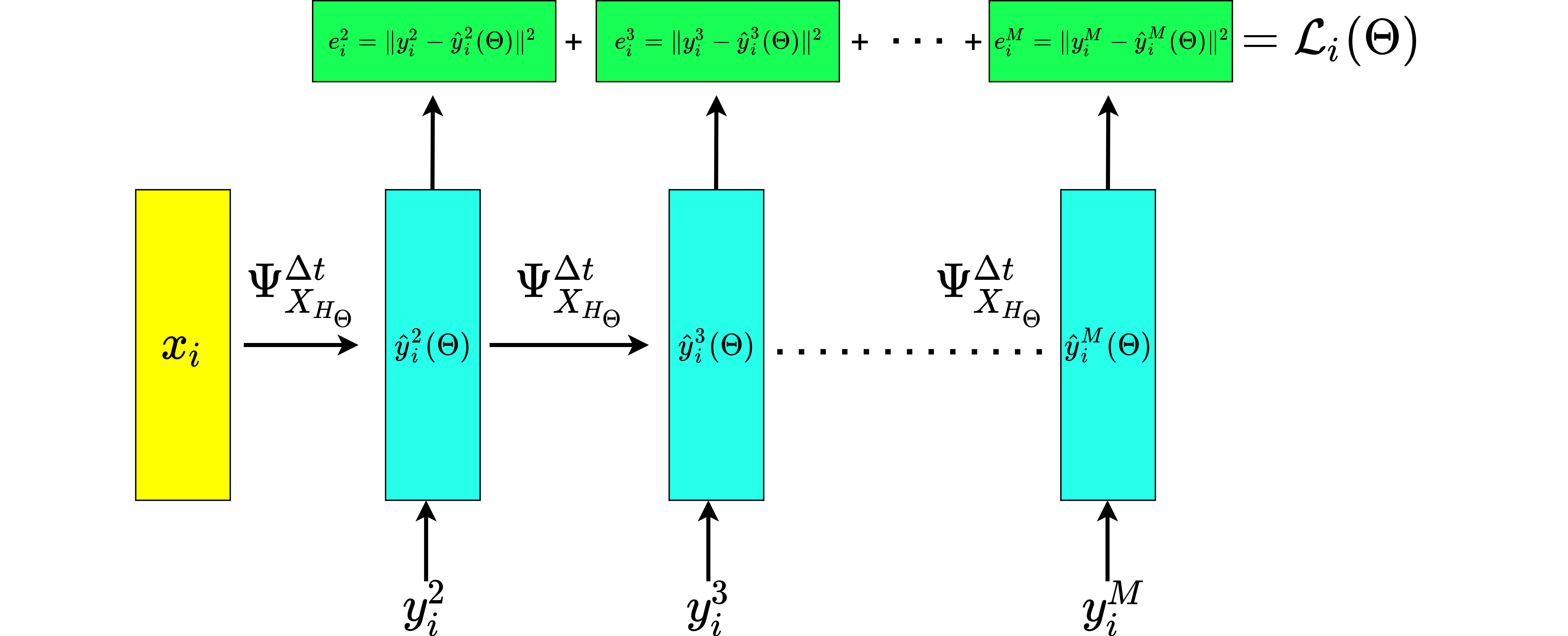
where \(\|\cdot\|\) is the Euclidean metric of \(\mathbb{R}^{2n}\). This is implemented with the PyTorch \(\texttt{MSELoss}\) loss function. Such a training procedure resembles the one of Recurrent Neural Networks (RNNs), as shown for the forward pass of a single training trajectory in the following figure.

Figure 1. Forward pass of an input training trajectory \((x_i,y_i^2,...,y_i^M)\). The picture highlights the resemblance to an unrolled version of a Recurrent Neural Network. The network outputs \((\hat{y}_i^2,…,\hat{y}_i^M)\).

Indeed, the weight sharing principle of RNNs is reproduced by the time steps in the numerical integrator which are all based on the same approximation of the Hamiltonian, and hence on the same weights \(\Theta\).

Architecture of the network

In this example, the role of the neural network is to model the Hamiltonian, i.e. a scalar function defined on the phase space \(\mathbb{R}^{2n}\). Thus, the starting and arrival spaces are fixed.

We leverage the form of the kinetic energy, where \(M(q)\) is modelled through a constant symmetric and positive definite matrix with entries \(m_{ij}\). Therefore, we aim at learning a constant matrix \(A\in\mathbb{R}^{k\times k}\) and a vector \(b\in\mathbb{R}^k\) so that

(4)\[\begin{split}\begin{align} \begin{bmatrix} m_{11} & ... & m_{1k}\\ m_{21} & ... & m_{2k}\\ \vdots & \vdots & \vdots \\ m_{k1} & ... & m_{kk} \end{bmatrix} \approx A^TA + \begin{bmatrix} \tilde{b}_{1} & 0 & ... & 0 \\ 0 & \tilde{b}_2 & \ddots & \vdots \\ \vdots & \ddots & \ddots & 0 \\ 0 & ... & 0 & \tilde{b}_k \end{bmatrix} \end{align}\end{split}\]

where \(\tilde{b}_i := \max{(0,b_i)}\) are terms added to promote the positive definiteness of the right-hand side. Notice that, in principle, the imposition of the positive (semi)definiteness of the matrix defining the kinetic energy is not necessary, but it allows to get more interpretable results. Indeed, it is known that the kinetic energy should define a metric on \(\mathbb{R}^n\) and the assumption we are making guarantees such a property. For the potential energy, a possible modelling strategy is to work with standard feedforward neural networks, and hence to define

(5)\[\begin{align} V(q) \approx V_{\theta}(q) = f_{\theta_m}\circ ...\circ f_{\theta_1}(q) \end{align}\]

(6)\[\begin{align} \theta_i = (W_i,b_i)\in\mathbb{R}^{n_i\times n_{i-1}}\times \mathbb{R}^{n_i},\;\theta:=[\theta_1,...,\theta_m], \end{align}\]

(7)\[\begin{align} f_{\theta_i}(u) := \Sigma(W_iu + b_i),\;\mathbb{R}^n\ni z\mapsto \Sigma(z) = [\sigma(z_1),...,\sigma(z_n)]\in\mathbb{R}^n, \end{align}\]

for example with \(\sigma(x) = \tanh(x)\). Therefore, we have that

(8)\[\begin{align} \Theta = [A, \theta], \quad H(q,p) \approx H_{\Theta}(q,p) = K_A(p) + V_{\theta}(q). \end{align}\]

The neural network for the parameterized Hamiltonian (8) is defined in the following PyTorch class.

class Learning_Hamiltonians.main.Hamiltonian

Class to define the neural network (parameterized Hamiltonian), which inherits from nn.Module

__init__()

Method where the parameters are defined

MassMat(X)

Mass matrix defining the kinetic energy quadratic function

Parameters:

X (torch.Tensor) – training trajectory points in input, with shape [batch size, nop*2s]

Returns:

row – Mass matrix to be learned by the neural network, with shape [batch size, nop*s, nop*s]

Return type:

torch.Tensor

Kinetic(X)

Kinetic energy in the Hamiltonian function

Parameters:

X (torch.Tensor) – training trajectory points in input, with shape [batch size, nop*2s]

Returns:

row – Kinetic energy, with shape [batch size, 1]

Return type:

torch.Tensor

Potential(X)

Potential energy in the Hamiltonian function

Parameters:

X (torch.Tensor) – training trajectory points in input, with shape [batch size, nop*2s]

Returns:

row – Potential energy, with shape [batch size, 1]

Return type:

torch.Tensor

forward(X)

Forward function that receives a tensor containing the input (trajectory points in the phase space) and returns a tensor containing a scalar output (Hamiltonian)).

Parameters:

X (torch.Tensor) – training trajectory points in input, with shape [batch size, nop*2s]

Returns:

o – Value of the Hamiltonian, with shape [batch size, 1]

Return type:

torch.Tensor