Example

Problem description

We consider a multibody system made of two cooperating quadrotor unmanned aerial vehicles (UAV) connected to a point mass (suspended load) via rigid links. This model is described in (Lee, Sreenath, Kumar, 2013).

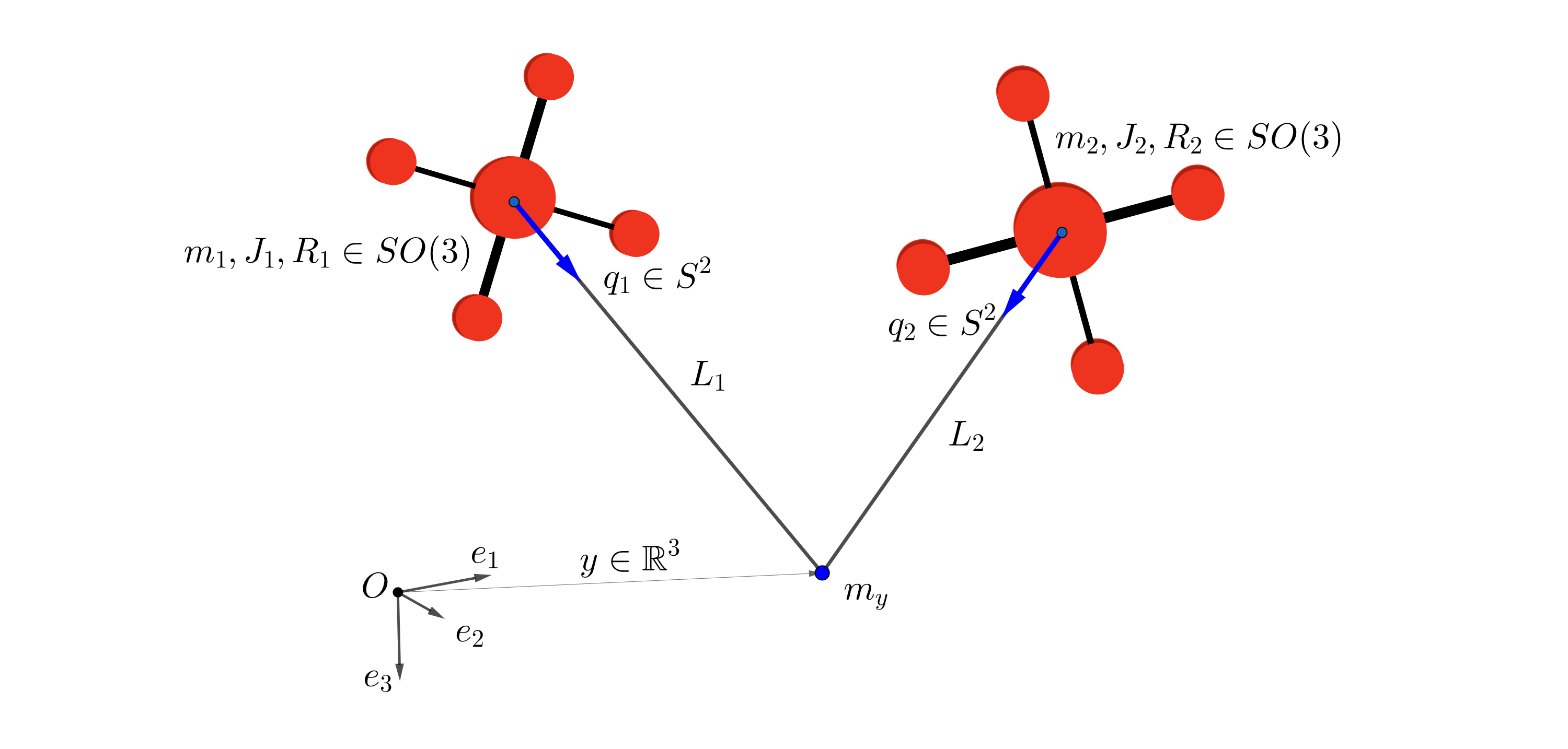
Figure 1. Two quadrotors connected to the mass point \(m_y\) via massless links of lengths \(L_i\).

We introduce an inertial frame whose third axis goes in the direction of gravity, but opposite orientation, and we attach body-fixed frames to each quadrotor (with the origins located respectively at the center of mass of each quadrotor). We denote with \(y,y_1,y_2\in\mathbb{R}^3\) the locations, respectively, of the mass point and the center of mass of each quadrotor with respect to the intertial frame. We assume that the links between the two quadrotors and the mass point are of a fixed length \(L_1, L_2\in\mathbb{R}^+\). The configuration variables of the system are: the position of the mass point in the inertial frame, \(y\in \mathbb{R}^3\), the attitude matrices of the two quadrotors, \((R_1, R_2)\in (SO(3))^2\) and the directions of the links which connect the center of mass of each quadrotor respectively with the mass point, \((q_1,q_2)\in (S^2)^2\). The configuration manifold of the system is

(1)\[\begin{align} Q=\mathbb{R}^3\times (SO(3))^2 \times (S^2)^2. \end{align}\]

In order to write the equations of motion of the system, we identify \(TSO(3)\simeq SO(3)\times \mathfrak{so}(3)\) via left-trivialization. This choice allows us to write the kinematic equations of the system as

(2)\[\begin{align} \dot{R}_i = R_i\hat{\Omega}_i,\quad \dot{q}_i = \hat{\omega}_iq_i,\quad \quad i=1,2, \end{align}\]

where \(\Omega_1,\Omega_2\in\mathbb{R}^3\) represent the angular velocities of each quadrotor expressed with respect to its body-fixed frame, and \(\omega_1,\omega_2\) are the angular velocities of the links \(q_1,q_2\in S^2\), satisfying \(q_i\cdot\omega_i=0\;(i=1,2)\). The hat map

(3)\[\begin{split}\hat{\cdot}:\mathbb{R}^3\rightarrow \mathfrak{so}(3),\qquad \begin{align} \xi=\left[\begin{array}{c} \xi_1 \\ \xi_2 \\ \xi_3 \end{array}\right] \rightarrow \hat{\xi}=\left[\begin{array}{ccc} 0 & -\xi_3 & \xi_2 \\ \xi_3 & 0 & -\xi_1 \\ -\xi_2 & \xi_1 & 0 \end{array}\right]\, \end{align}\end{split}\]

is such that \(\hat{a}b=a\times b\) for all \(a,\,b\in \mathbb{R}^3\). This allows us to identify elements of the lie algebra \(\mathfrak{so}(3)\), modelled as \(3\times3\) skew symmetric matrices, with vectors in \(\mathbb{R}^3\).

We define the trivialized Lagrangian

(4)\[\begin{align} L(y,\dot{y},R_1,\Omega_1,R_2,\Omega_2,q_1,\omega_1,q_2,\omega_2): \mathbb{R}^6\times \left(SO(3)\times \mathfrak{so}(3)\right)^2\times (TS^2)^2\rightarrow \mathbb{R}, \end{align}\]

as the difference of the total kinetic energy of the system and the total potential (gravitational) energy, \(L=T-U\), with:

(5)\[\begin{align} T = \frac{1}{2}m_y\|\dot{y}\|^2 +\frac{1}{2}\sum_{i=1}^2 (m_i\|\dot{y} -L_i\hat{\omega}_iq_i \|^2 + \Omega_i^TJ_i\Omega_i) , \end{align}\]

and

(6)\[\begin{align} U= -m_yge_3^Ty - \sum_{i=1}^2 m_ige_3^T(y-L_iq_i), \end{align}\]

where \(J_1,J_2\in\mathbb{R}^{3\times 3}\) are the inertia matrices of the two quadrotors and \(m_1,m_2\in\mathbb{R}^+\) are their respective total masses. In this system each of the two quadrotors generates a thrust force \(u_i = -T_iR_ie_3\in\mathbb{R}^3\,(i=1,2)\) with respect to the inertial frame, with \(T_i\) the thrust magnitude and \(e_3\) the direction of the thrust vector in the i-th body-fixed frame. The presence of these forces make it a non conservative system. Moreover, the rotors of each of the two quadrotors generate a moment vector with respect to its body-fixed frame, and we denote with \(M_1, M_2\in\mathbb{R}^3\) the cumulative moment vector of each of the two quadrotors. By using the Lagrange–d’Alambert’s principle, we get the following Euler–Lagrange equations:

(7)\[\begin{align} A(z)\dot{z} = h(z) \end{align}\]

where

(8)\[\begin{align} z = [y,v,\Omega_1,\Omega_2,\omega_1,\omega_2]^T\in\mathbb{R}^{18}, \end{align}\]

(9)\[\begin{split}\begin{align} A(z) = \begin{bmatrix} I_3 & 0_3 & 0_3 & 0_3 & 0_3 & 0_3 \\ 0_3 & M_q & 0_3 & 0_3 & 0_3 & 0_3 \\ 0_3 & 0_3 & J_1 & 0_3 & 0_3 & 0_3 \\ 0_3 & 0_3 & 0_3 & J_2 & 0_3 & 0_3 \\ 0_3 & -\frac{1}{L_1}\hat{q}_1 & 0_3 & 0_3 & I_3 & 0_3 \\ 0_3 & -\frac{1}{L_2}\hat{q}_2 & 0_3 & 0_3 & 0_3 & I_3\end{bmatrix}, \end{align}\end{split}\]

(10)\[\begin{split}\begin{align} h(z) = \begin{bmatrix}h_1(z) \\ h_2(z) \\ h_3(z) \\ h_4(z) \\ h_5(z) \\ h_6(z)\end{bmatrix} =\begin{bmatrix} v \\ -\sum_{i=1}^{2} m_{i}L_{i}\|\omega_{i} \|^{2} q_{i} + M_q g e_{3}+\sum_{i=1}^{2} u_i^{\parallel} \\ -\Omega_1\times J_1\Omega_1 + M_1 \\ -\Omega_2\times J_2\Omega_2 + M_2 \\ -\frac{1}{L_1} g \hat{q}_{1} e_{3} -\frac{1}{m_1L_1}q_{1} \times u_1^{\perp}\\ -\frac{1}{L_2} g \hat{q}_{2} e_{3} -\frac{1}{m_2L_2}q_{2} \times u_2^{\perp}\end{bmatrix}, \end{align}\end{split}\]

where \(M_q = m_yI_3 + \sum_{i=1}^2m_iq_iq_i^T,\) and \(u_i^{\parallel},u_i^{\perp}\) are respectively the orthogonal projection of \(u_i\) along \(q_i\) and to the plane \(T_{q_i}S^2\), \(i=1,2\), i.e. \(u_i^{\parallel}=q_{i} q_{i}^{T}u_i\), \(u_i^{\perp}=(I-q_{i} q_{i}^{T})u_i\). These equations, coupled with the kinematic equations, describe the dynamics of a point

(11)\[\begin{align} P = \left[y ,\;\; v,\;\; R_1 ,\;\; \Omega_1 ,\;\; R_2 ,\;\; \Omega_2 ,\;\; q_1 ,\;\; \omega_1 ,\;\; q_2 ,\;\; \omega_2 \right] \in \mathcal{M} = TQ. \end{align}\]

Since the matrix \(A(z)\) is invertible, we pass to the following set of equations

(12)\[\begin{align} \dot{z} = A^{-1}(z)h(z):=\tilde{h}(z) :=\bar{h}(P) = [\bar{h}_1(P),...,\bar{h}_6(P)]^T. \end{align}\]

We highlight that the inputs \(\{u_i^{\parallel},u_i^{\perp},M_i\}_{i=1,2}\) act as controls. They are constructed such that the point mass asymptotically follows a given desired trajectory \(y_d \in \mathbb{R}^3\), given by a smooth function of time, and the quadrotors maintain a prescribed formation relative to the point mass. In particular, the parallel components \(u_i^{\parallel}\) are designed such that the payload follows the desired trajectory \(y_d\) (load transportation problem), while the normal components \(u_i^{\perp}\) are designed such that \(q_i\) converge to desired directions \(q_{id}\) (tracking problem in \(S^2\)). Finally, \(M_i\) are designed to control the attitude of the quadrotors.

Analysis via transitive group action

In this section we show how to obtain the local representation of the vector field \(F\in\mathfrak{X}(\mathcal{M})\) of the system presented above in terms of the infinitesimal generator of a transitive group action \(\psi\), as described in the section Algorithms. This is the formalism also used in the main code. We start by identifying the phase space \(\mathcal{M}\) with

(13)\[\begin{align} \mathcal{M}\simeq T\mathbb{R}^3\times (TSO(3))^2 \times (TS^2)^2. \end{align}\]

The group we consider is

(14)\[\begin{align} \bar{G} = \mathbb{R}^6 \times (TSO(3))^2 \times (SE(3))^2, \end{align}\]

where the groups are combined with a direct-product structure and \(\mathbb{R}^6\) is the additive group. For a group element

(15)\[\begin{align} g=((a_1,a_2),((B_1,b_1),(B_2,b_2)),((C_1,c_1),(C_2,c_2)))\in \bar{G} \end{align}\]

and a point \(P \in \mathcal{M}\) in the manifold, we consider the following left action

(16)\[\begin{split}\begin{align} \begin{split} \psi_g(P) = [y+a_1, \;\;v+a_2,\;\; &B_1R_1,\;\; \Omega_1 + b_1,\;\; B_2R_2,\;\; \Omega_2 + b_2,\;\;\\ &C_1q_1,\;\;C_1\omega_1 + c_1\times C_1q_1,\;\; C_2q_2,\;\;C_2\omega_2 + c_2\times C_2q_2]. \end{split} \end{align}\end{split}\]

It can be proved that this is a well-defined and transitive action of \(\bar{G}\) on \(\mathcal{M}\). The infinitesimal generator associated to

(17)\[\begin{align} \xi = \left[\xi_1 ,\;\; \xi_2,\;\; \eta_1 ,\;\; \eta_2 ,\;\; \eta_3 ,\;\; \eta_4 ,\;\; \mu_1 ,\;\; \mu_2 ,\;\; \mu_3 ,\;\; \mu_4 \right]\in \mathfrak{\bar{g}}, \end{align}\]

where \(\mathfrak{\bar{g}}=T_e\bar{G}\), writes

(18)\[\begin{split}\begin{align} \begin{split} \psi_{*}(\xi)\vert_P = [\xi_1,\;\; \xi_2, \;\; \hat{\eta}_1R_1,\;\; \eta_2,\;\; &\hat{\eta}_3R_2,\;\; \eta_4,\;\;\\ & \hat{\mu}_1q_1,\;\; \hat{\mu}_1\omega_1 + \hat{\mu}_2q_1, \;\; \hat{\mu}_3q_2,\;\; \hat{\mu}_3\omega_2 + \hat{\mu}_4q_2 ]. \end{split} \end{align}\end{split}\]

We can now construct the function \(f:\mathcal{M}\rightarrow \bar{\mathfrak{g}}\) such that \(\psi_{*}(f(P))\vert_P=F\vert_P\), where

(19)\[\begin{split}\begin{align} \begin{split} F\vert_P = [\bar{h}_1(P), \;\; \bar{h}_2(P), \;\; R_1&\hat{\Omega}_1,\;\; \bar{h}_3(P), \;\; R_2\hat{\Omega}_2,\;\;\\ &\bar{h}_4(P), \;\; \hat{\omega}_1q_1, \;\; \bar{h}_5(P),\;\; \hat{\omega}_2q_2, \;\; \bar{h}_6(P)]\in T_{P}\mathcal{M} \end{split} \end{align}\end{split}\]

is the vector field obtained combining the kinematic and dynamic equations of motion. We have

(20)\[\begin{split}\begin{align} \begin{split} f(P) = [\bar{h}_1(P),\;\; \bar{h}_2(P),\;\; R_1\Omega_1,\;\;&\bar{h}_3(P),\;\; R_2\Omega_2,\;\;\bar{h}_4(P),\\ \;\;&\omega_1,\;\; q_1\times \bar{h}_5(P),\;\;\omega_2,\;\; q_2\times \bar{h}_6(P)]\in\bar{\mathfrak{g}}. \end{split} \end{align}\end{split}\]