Space-time discretisation

The space-time domain \(X\) is discretised as a rectangular grid \(X_d\) with \(N\) steps of length \(\Delta x\) in space and \(K\) steps of length \(\Delta t\) in time.

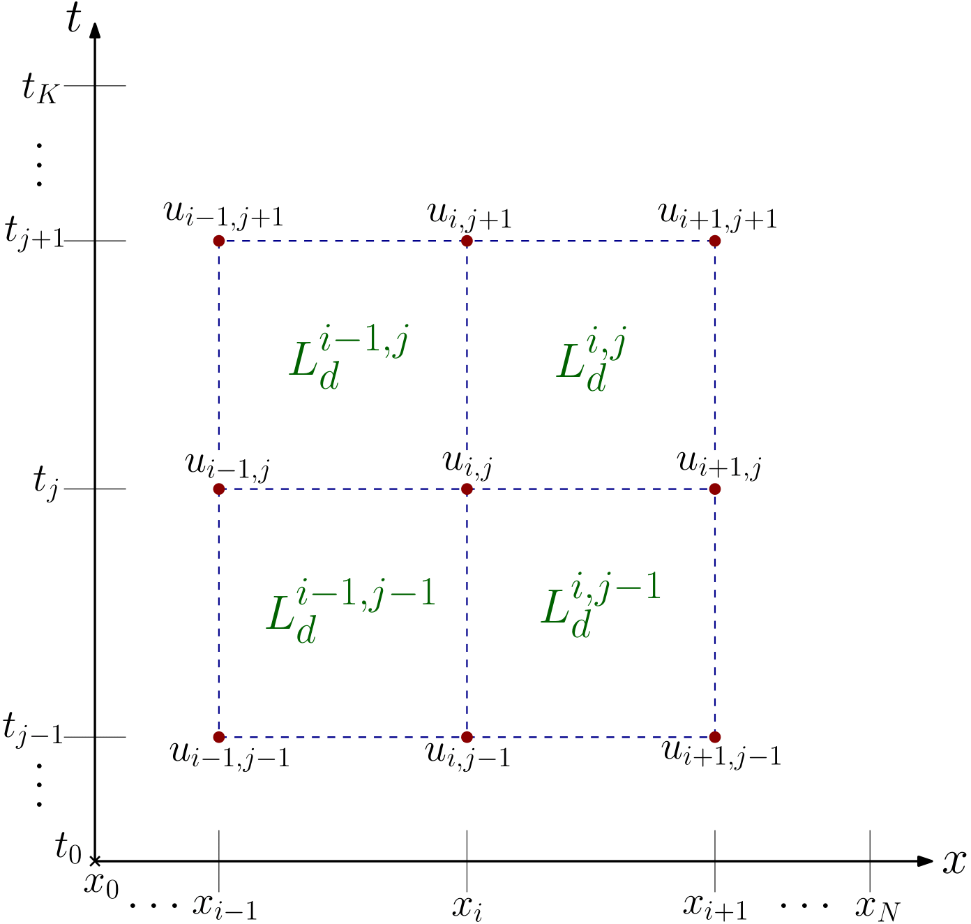
Figure 1. Discretised space-time domain with the representation of transverse deformations and discrete Lagrangians

The field is, thus, discretised by an indexed collection \(u_d = \{ u_{i,j} \in \mathbb{R} \;\vert\; i = 0, \dots, N,\, j = 0, \dots, K\}\). For each rectangular element with nodes \(\square_{i,j} = \{ (i,j), (i+1, j), (i, j+1), (i+1, j+1)\}\), we have a discrete Lagrangian \(L_d \,:\, \square_{i,j} \to \mathbb{R}\), \(L_d \left(u_{i,j},u_{i+1,j},u_{i,j+1},u_{i+1,j+1} \right)\), abbreviated as \(L^{i,j}_d\).

The trapezoidal quadrature rule is used to approximate the continuous action over each rectangle \(\square_{i,j}\). Then:

\[\begin{aligned} L^{i,j}_d = \frac{\Delta x \Delta t}{4} \left\{ \left( \frac{u_{i,j+1}-u_{i,j}}{\Delta t} \right)^2 + \left( \frac{u_{i+1,j+1}-u_{i+1,j}}{\Delta t} \right)^2 - c^2 \left[ \left( \frac{u_{i+1,j}-u_{i,j}}{\Delta x} \right)^2 + \left( \frac{u_{i+1,j+1}-u_{i,j+1}}{\Delta x} \right)^2 \right] \right\} \end{aligned}\]

The associated discrete action is:

\[\begin{align*} S_d[u_d] = \sum_{i=0}^{N-1} {\sum_{j=0}^{K-1} {L_d^{i,j}}} \end{align*}\]

The discrete solution field satisfies a discretised version of Hamilton’s principle. In other words, discrete physical trajectories are stationary points of the associated discrete action. The resulting discrete Euler-Lagrange equations at node \((i,j)\) are:

\[\begin{aligned} D_4 L^{i-1,j-1}_d + D_3 L^{i,j-1}_d + D_2 L^{i-1,j}_d + D_1 L^{i,j}_d = 0 \end{aligned}\]

Notice that these involve the discrete Lagrangians of all the rectangles containing \((i,j)\).

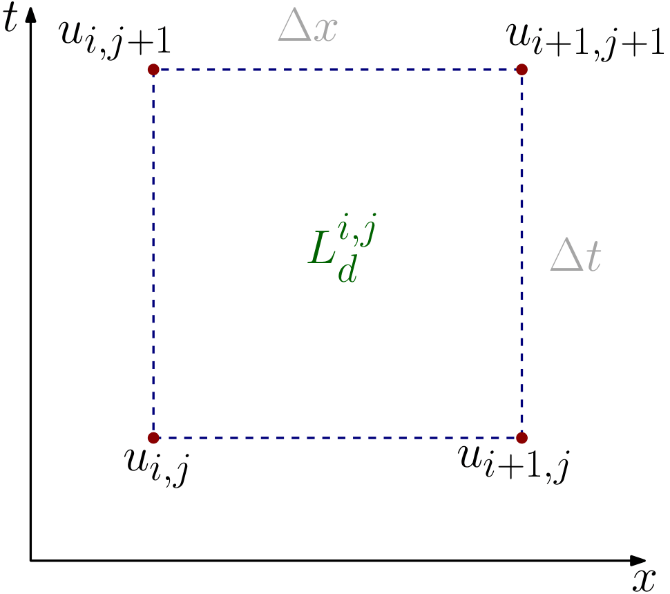
Figure 3. Discrete Lagrangian in the space-time domain

Boundary conditions

At the boundaries, initial (for \(t = 0\)) and boundary conditions (for \(x = 0\) and \(x = l\)) need to be taken into account to solve the problem.

To implement these, it is important to understand the meaning of the derivatives \(D_k L^{i,j}_d\), \(k = 1, \dots, 4\) and their relation to the canonical momenta, see the picture below. In our case, these derivatives can be interpreted as

\[\begin{split}\begin{aligned} D_1 L^{i,j}_d &= -\frac{\Delta t}{2} p_x^{i,j} - \frac{\Delta x}{2} p_t^{i,j}\\ D_2 L^{i,j}_d &= \frac{\Delta t}{2} p_x^{i+1,j} - \frac{\Delta x}{2} p_t^{i+1,j}\\ D_3 L^{i,j}_d &= -\frac{\Delta t}{2} p_x^{i,j+1} + \frac{\Delta x}{2} p_t^{i,j+1}\\ D_4 L^{i,j}_d &= \frac{\Delta t}{2} p_x^{i+1,j+1} + \frac{\Delta x}{2} p_t^{i+1,j+1}\\ \end{aligned}\end{split}\]

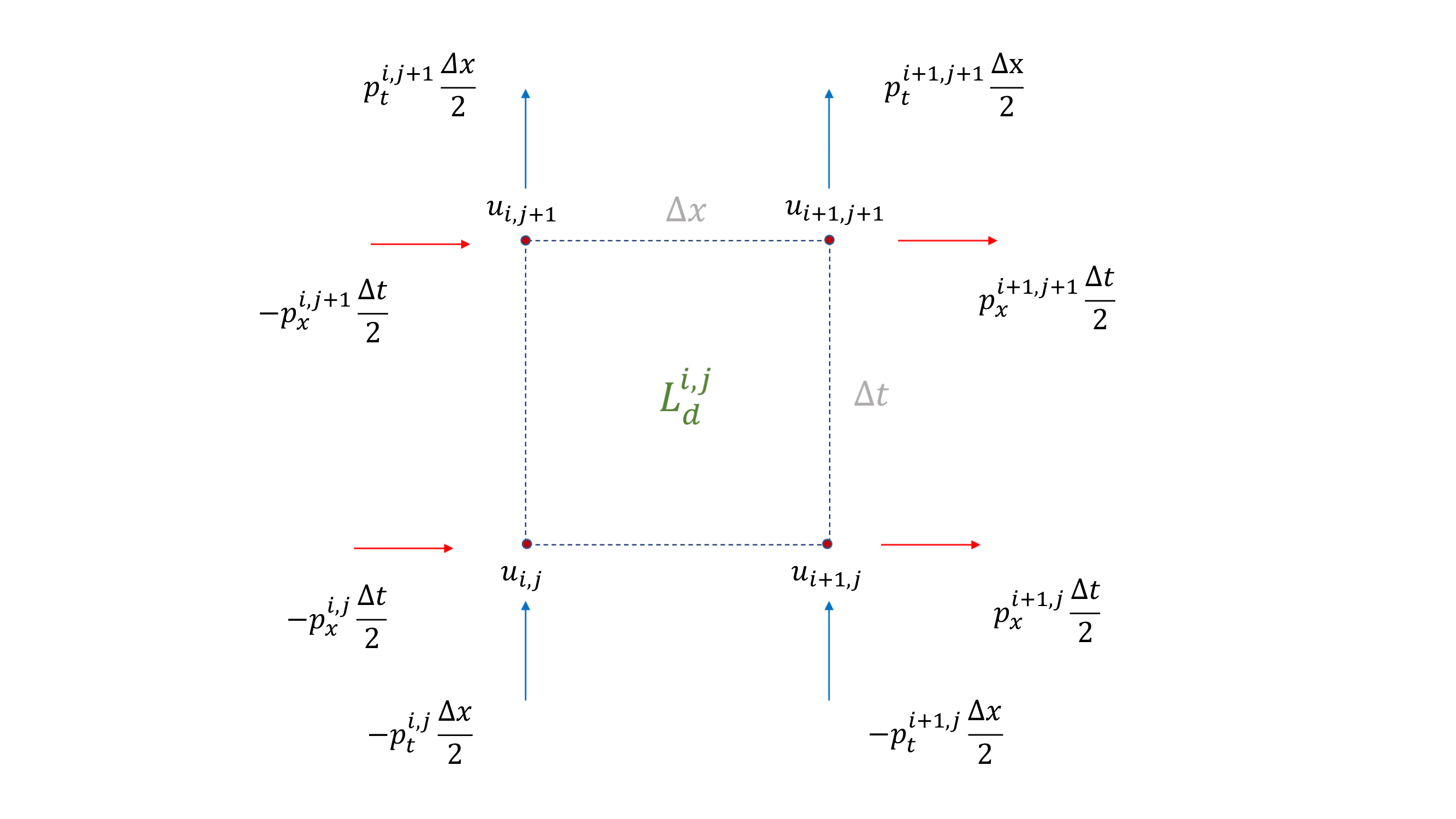
Figure 2. Representation of the momenta in the space-time domain

Currently, the following conditions are hardcoded:

\[\begin{split}\begin{aligned} u(x,0) &= \sin(\pi x)\\ \dot{u}(x,0) &= 0\\ u(0,t) &= 0\\ u(l,t) &= 0 \end{aligned}\end{split}\]

To implement the first, all nodes \(u_{i,0}\) have been fixed to their corresponding values, \(\sin(\pi i \Delta x)\), and for the latter two, \(u_{0,j}\) and \(u_{N,j}\) have been set to zero. To implement the second, we make use of the above interpretation to write and solve the equations,

\[\begin{aligned} D_2 L^{i-1,0}_d + D_1 L^{i,0}_d + \Delta s p_t^{i,0} = 0, \quad i = 1,\dots,N-1 \end{aligned}\]

where, in our case, \(p_t = \dot{u}\).