Post-processing and results

Results are shown in terms of:

• energy density, i.e. the energy of the system is evaluated at each node of the beam during the whole simulation time as:

  \[\begin{aligned} H_{density} \left( x,t,u,\dot{u},u' \right) = \frac{1}{2} \left( \dot{u}^2 + c^2 u' ^2 \right) \end{aligned}\]

• energy charge, i.e. the total energy of the system evaluated in the discretised simulation time

  \[\begin{aligned} H_{charge} \left( t \right) = \int_{0}^l \left[ \frac{1}{2} \left( u' ^2 + c^2 \dot{u}^2 \right) dx \right] \end{aligned}\]

Both quantities are calculated by using the discrete Legendre transform. In the discrete settings, energy density and charge are respectively detemined as follow:

\[\begin{aligned} H_{density}^{i,j} = \frac{1}{2} \left( (p_t^{i,j})^2 + c^2 (p_x^{i,j})^2 \right) \; \; \text{for} \; i=0 \dots l \text{,} \; j=0 \dots \tau \end{aligned}\]

\[\begin{aligned} H_{charge}^j = \sum\limits_{i=0}^l \left[ \frac{1}{2} \left( (p_t^{i})^2 + c^2 (p_x^{i})^2 \right) \right] \; \text{for} \; j=0 \dots \tau \end{aligned}\]

In the 1D_wave_equation, the energy density is evaluated as follow:

for j=1:n_t
     for i=1:n_s
         T_kin(i,j) = 1/2*rho*pp_t(i,j)^2;
         V_pot(i,j) = 1/2*k_pot*pp_s(i,j)^2;
         HH(i,j) = T_kin(i,j)+V_pot(i,j);
         HH_charge_node(i,j) = 1/2*(pp_t(i,j)^2+k_pot/rho*pp_s(i,j)^2);
         if not(i == 1)
         HH_charge_elem(i-1,j) = 1/2*delta_s*(HH_charge_node(i-1,j)+HH_charge_node(i,j));
         end
     end
 end

where n_t is the number of time steps, n_s is the number of nodes, T_kin is the kinetic energy, V_pot is the potential energy, rho is the density and k_pot is the modulus of elasticity of the string. Moreover, instead of computing the energy charge itself, in the Matlab code its error during simulation is evaluated.

for j=1:n_t
    HH_charge(j) = sum(HH_charge_elem(:,j));
    HH_error(j) = HH_charge(1)-HH_charge(j);
end

For the particular example problem, the above quantities are shown in Figure 1 and 2. It can be notice the good behaviour of the energy charge with an error in time of the order of \(10^{-15}\) in Figure 2.

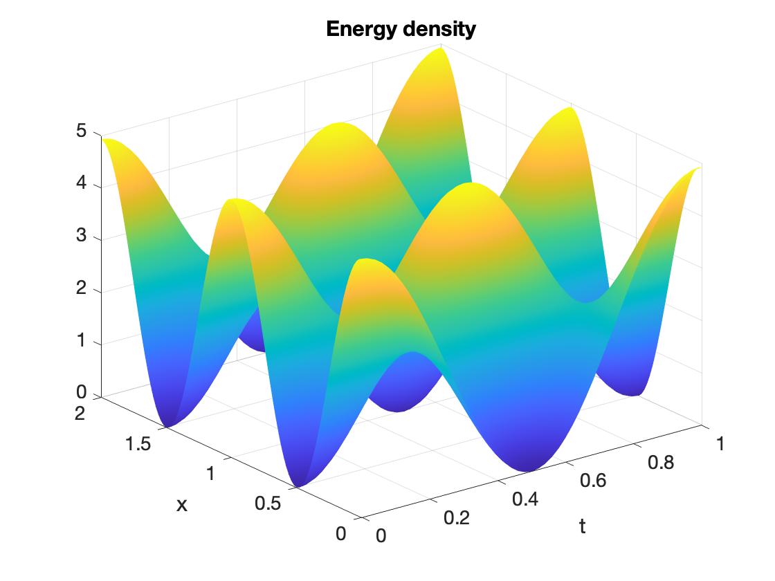
Figure 1. Energy density

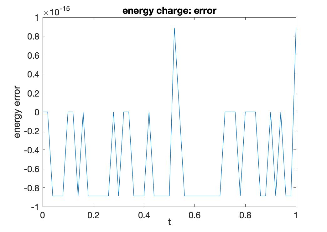
Figure 2. Energy charge: error